Finished Mathematics for Computer Science class

Today I finally finished the Mathematics for Computer Science class that I have worked on since December. For the last year or two I have wanted to do some general Computer Science study in my free time that is not directly related to my work. I documented a lot of this journey in an earlier blog post.

The math class is on MIT’s OpenCourseWare (OCW) web site. It was an undergraduate semester class and I spent about 9 months on it mostly in my spare time outside of work. I wanted to test out OCW as a source for training just as I had experimented with edX before. So, I thought I would share my thoughts on the experience.

The class contained high quality material. It was an undergraduate class so it may not have been as deep as a graduate level class could be but world-class MIT professors taught the class. Some of my favorite parts of the video lectures were where professor Leighton made comments about how the material applied in the real world.

The biggest negative was that a lot of the problems did not have answers. Also, I was pretty much working through this class on my own. There were some helpful people on a Facebook group that some of my edX classmates created that helped keep me motivated. But there wasn’t a large community of people taking the same class.

Also, it makes me wonder where I should spend time developing myself. Should I be working more on my communication and leadership skills through Toastmasters? Should I be working on my writing? Should I be learning more Oracle features?

I spent months studying for Oracle’s 12c OCP certification exam and I kind of got burnt out on that type of study. The OCP exam has a lot of syntax. To me syntax, which you can look up in a manual, is boring. The underlying computer science is interesting. It is fun to try to understand the Oracle optimizer and Oracle internals, locking, backup and recovery, etc. There is a never-ending well of Oracle knowledge that I could pursue.

Also, there is a lot of cloud stuff going on. I could dive into Amazon and other cloud providers. I also have an interest in open source. MySQL and PostgreSQL intrigue me because I could actually have the source code.

But, there is only so much time in the day and I can’t do everything. I don’t regret taking the math for computer science class even if it was a diversion from my Toastmasters activities and not directly related to work. Now I have a feel for the kind of materials that you have on OCW: high quality, general computer science, mostly self-directed. Now I just have to think about what is next.

Bobby

Posted in Uncategorized | 2 Comments

Trying VirtualBox

I have been using  VMware Player to build test virtual machines on my laptop with an external drive for some time now. I used to use the free VMware Server. My test VMs weren’t fast because of the slow disk drive but they were good enough to run small Linux VMs to evaluate software. I also had one VM to do some C hacking of the game Nethack for fun. I got a lot of good use out of these free VMware products and VMware is a great company so I’m not knocking them. But, this week I accidentally wiped out all the VMs that I had on my external drive so I tried to rebuild one so I at least have one to boot up if I need a test Linux VM. I spend several hours trying to get the Oracle Linux 6.8 VM that I created to work with a screen resolution that matched my monitor. I have a laptop with a smaller 14 inch 1366 x 768 resolution built-in monitor and a nice new 27 inch 1920 x 1080 resolution external monitor. VMware player wouldn’t let me set the resolution to more than 1366 x 768 no matter what I did.

Finally after a lot of googling and trying all kinds of X Windows and VMware settings I finally gave up and decided to try VirtualBox. I was able to quickly install it and get my OEL 6.8 VM up with a larger resolution with no problem. It still didn’t give me 1920 x 1080 for some reason but had a variety of large resolutions to choose from.

After getting my Linux 6.8 machine to work acceptably I remembered that I was not able to get Linux 7 to run on VMware either. I had wanted to build a VM with the latest Linux but couldn’t get it to install. So, I downloaded the 7.2 iso and voilà it installed like a charm in VirtualBox. Plus I was able to set the resolution to exactly 1920 x 1080 and run in full screen mode taking up my entire 27 inch monitor.  Very nice!

I have not yet tried it, but VirtualBox seems to come with the ability to take a snapshot of a VM and to clone a VM. To get these features on VMware I’m pretty sure you need to buy the $249 VMware Workstation. I have a feeling that Workstation is a good product but I think it makes sense to try VirtualBox and see if the features that it comes with meet all my needs.

I installed VirtualBox at the end of the work day today so I haven’t had a lot of time to find its weaknesses and limitations. But so far it seems to have addressed several weaknesses that I found in VMware Player so it may have a lot of value to me. I think it is definitely worth trying out before moving on to the commercial version of VMware.

Bobby

P.S. Just tried the snapshot and clone features. Very neat. Also I forgot another nuisance with VMware Player. It always took a long time to shut down a machine. I think it was saving the current state. I didn’t really care about saving the state or whatever it was doing. Usually I just wanted to bring something up real quick and shut it down fast. This works like a charm on VirtualBox. It shuts down a VM in seconds. So far so good with VirtualBox.

P.P.S This morning I easily got both my Linux 6.8 and 7.2 VM’s to run with a nice screen size that takes up my entire 27 inch monitor but leaves room so I can see the menu at the top of the VM window and my Windows 7 status bar below the VM’s console window. Very nice. I was up late last night tossing and turning in bed thinking about all that I could do with the snapshot and linked clone features. 🙂

P.P.P.S. Now the bad news. Virtualbox is not working for me with USB flash drives. This works flawlessly out of the box with VMware player. I guess it was inevitable that I would find things that VMware does better. Maybe VMware works better with Windows hosts. I seem to be hitting this issue. It seems to be a known bug using USB flash drives on Windows 7 using Virtualbox. Seems to have been a bug for about 4 years. The workaround seems to be to edit the registry on my work laptop. Not going to do that.

Posted in Uncategorized | 2 Comments

Modified IO CPU+IO Elapsed Graph (sigscpuio)

Still tweaking my Python based Oracle database performance tuning graphs.

I kind of like this new version of my “sigscpuio” graph:

blogiopluscp2u

The earlier version plotted IO, CPU, and Elapsed time summed over a group of force matching signatures. It showed the components of the time spent by the SQL statements represented by those signatures. But the IO and CPU lines overlapped and you really could not tell how the elapsed time related to IO and CPU.  I thought of changing to a stacked graph where the graph layered all three on top of each other but that would not work. Elapsed time is a separate measure of the total wall clock time and could be more or less than the total IO and CPU time. So, I got the idea of tweaking the chart to show IO time on the bottom, CPU+IO time in the middle, and let the line for elapsed time go wherever it falls. It could be above the CPU+IO line if there was time spent that was neither CPU or IO. It could fall below the line if CPU+IO added up to more than the elapsed time.

So, this version of sigscpuio kind of stacks CPU and IO and just plots elapsed time wherever it falls.  Might come in handy.

Bobby

Posted in Uncategorized | Leave a comment

Graph frequently executed SQL by FORCE_MATCHING_SIGNATURE

I made a new graph in my PythonDBAGraphs program. Here is an example with real data but the database name blanked out:

sql_matching_group_of_signatures_blog

My graphs are all sized for 1920 x 1080 monitors so I can see all the detail in the lines using my entire screen. The idea for this graph is to show how the performance of the queries that matter to the users changes as we add more load and data to this production database. I knew that this database had many queries with literals in their where clauses. I decided to pick a group of SQL by FORCE_MATCHING_SIGNATURE and to graph the average elapsed run time against the total number of executions.

I used this query to list all the SQL by signature:

column FORCE_MATCHING_SIGNATURE format 99999999999999999999

select FORCE_MATCHING_SIGNATURE,
sum(ELAPSED_TIME_DELTA)/1000000 total_seconds,
sum(executions_delta) total_executions,
count(distinct sql_id) number_sqlids,
count(distinct snap_id) number_hours,
min(PARSING_SCHEMA_NAME)
from DBA_HIST_SQLSTAT
group by FORCE_MATCHING_SIGNATURE
order by number_hours desc;

This is an edited version of the output – cut down to fit the page:

FORCE_MATCHING_SIGNATURE TOTAL_SECONDS TOTAL_EXECUTIONS NUMBER_HOURS
------------------------ ------------- ---------------- ------------
    14038313233049026256     22621.203         68687024         1019
    18385146879684525921    18020.9776        157888956         1013
     2974462313782736551    22875.4743           673687          993
    12492389898598272683    6203.78985         66412941          992
    14164303807833460050    4390.32324           198997          980
    10252833433610975622    6166.07675           306373          979
    17697983043057986874    17391.0907         25914398          974
    15459941437096211273    9869.31961          7752698          967
     2690518030862682918    15308.8561          5083672          952
     1852474737868084795    50095.5382          3906220          948
     6256114255890028779    380.095915          4543306          947
    16226347765919129545    9199.14289           215756          946
    13558933806438570935    394.913411          4121336          945
    12227994223267192558    369.784714          3970052          945
    18298186003132032869    296.887075          3527130          945
    17898820371160082776    184.125159          3527322          944
    10790121820101128903    2474.15195          4923888          943
     2308739084210563004    265.395538          3839998          941
    13580764457377834041    2807.68503         62923457          934
    12635549236735416450    1023.42959           702076          918
    17930064579773119626    2423.03972         61576984          914
    14879486686694324607     33.253284            17969          899
     9212708781170196788     7292.5267           126641          899
      357347690345658614    6321.51612           182371          899
    15436428048766097389     11986.082           334125          886
     5089204714765300123    6858.98913           190700          851
    11165399311873161545    4864.60469         45897756          837
    12042794039346605265    11223.0792           179064          835
    15927676903549361476    505.624771          3717196          832
     9120348263769454156    12953.0746           230090          828
    10517599934976061598     311.61394          3751259          813
     6987137087681155918    540.565595          3504784          809
    11181311136166944889      5018.309         59540417          808
      187803040686893225    3199.87327         12788206          800

I picked the ones that had executed in 800 or more hours. Our AWR has about 1000 hours of history so 800 hours represents about 80% of the AWR snapshots. I ended up pulling one of these queries out because it was a select for update and sometimes gets hung on row locks and skews the graph. So, the graph above has that one pulled out.

I based the graph above on this query:

select
sn.END_INTERVAL_TIME,
sum(ss.executions_delta) total_executions,
sum(ELAPSED_TIME_DELTA)/((sum(executions_delta)+1))
from DBA_HIST_SQLSTAT ss,DBA_HIST_SNAPSHOT sn
where ss.snap_id=sn.snap_id
and ss.INSTANCE_NUMBER=sn.INSTANCE_NUMBER
and ss.FORCE_MATCHING_SIGNATURE in
(
14038313233049026256,
18385146879684525921,
2974462313782736551,
12492389898598272683,
14164303807833460050,
10252833433610975622,
17697983043057986874,
15459941437096211273,
2690518030862682918,
6256114255890028779,
16226347765919129545,
13558933806438570935,
12227994223267192558,
18298186003132032869,
17898820371160082776,
10790121820101128903,
2308739084210563004,
13580764457377834041,
12635549236735416450,
17930064579773119626,
14879486686694324607,
9212708781170196788,
357347690345658614,
15436428048766097389,
5089204714765300123,
11165399311873161545,
12042794039346605265,
15927676903549361476,
9120348263769454156,
10517599934976061598,
6987137087681155918,
11181311136166944889,
187803040686893225
)
group by sn.END_INTERVAL_TIME
order by sn.END_INTERVAL_TIME;

Only time will tell if this really is a helpful way to check system performance as the load grows, but I thought it was worth sharing what I had done. Some part of this might be helpful to others.

Bobby

Posted in Uncategorized | Leave a comment

Understanding query slowness after platform change

We are moving a production database from 10.2 Oracle on HP-UX 64 bit Itanium to 11.2 Oracle on Linux on 64 bit Intel x86. So, we are upgrading the database software from 10.2 to 11.2. We are also changing endianness from Itanium’s byte order to that of Intel’s x86-64 processors. Also, my tests have shown that the new processors are about twice as fast as the older Itanium CPUs.

Two SQL queries stand out as being a lot slower on the new system although other queries are fine. So, I tried to understand why these particular queries were slower. I will just talk about one query since we saw similar behavior for both. This query has sql_id = aktyyckj710a3.

First I looked at the way the query executed on both systems using a query like this:

select ss.sql_id,
ss.plan_hash_value,
sn.END_INTERVAL_TIME,
ss.executions_delta,
ELAPSED_TIME_DELTA/(executions_delta*1000),
CPU_TIME_DELTA/(executions_delta*1000),
IOWAIT_DELTA/(executions_delta*1000),
CLWAIT_DELTA/(executions_delta*1000),
APWAIT_DELTA/(executions_delta*1000),
CCWAIT_DELTA/(executions_delta*1000),
BUFFER_GETS_DELTA/executions_delta,
DISK_READS_DELTA/executions_delta,
ROWS_PROCESSED_DELTA/executions_delta
from DBA_HIST_SQLSTAT ss,DBA_HIST_SNAPSHOT sn
where ss.sql_id = 'aktyyckj710a3'
and ss.snap_id=sn.snap_id
and executions_delta > 0
and ss.INSTANCE_NUMBER=sn.INSTANCE_NUMBER
order by ss.snap_id,ss.sql_id;

It had a single plan on production and averaged a few seconds per execution:

PLAN_HASH_VALUE END_INTERVAL_TIME         EXECUTIONS_DELTA Elapsed Average ms CPU Average ms IO Average ms Cluster Average ms Application Average ms Concurrency Average ms Average buffer gets Average disk reads Average rows processed
--------------- ------------------------- ---------------- ------------------ -------------- ------------- ------------------ ---------------------- ---------------------- ------------------- ------------------ ----------------------
      918231698 11-MAY-16 06.00.40.980 PM              195         1364.80228     609.183405    831.563728                  0                      0                      0          35211.9487             1622.4             6974.40513
      918231698 11-MAY-16 07.00.53.532 PM              129         555.981481     144.348698    441.670271                  0                      0                      0          8682.84496         646.984496             1810.51938
      918231698 11-MAY-16 08.00.05.513 PM               39         91.5794872     39.6675128    54.4575897                  0                      0                      0          3055.17949          63.025641             669.153846
      918231698 12-MAY-16 08.00.32.814 AM               35         178.688971     28.0369429    159.676629                  0                      0                      0          1464.28571              190.8             311.485714
      918231698 12-MAY-16 09.00.44.997 AM              124         649.370258     194.895944    486.875758                  0                      0                      0           13447.871         652.806452             2930.23387
      918231698 12-MAY-16 10.00.57.199 AM              168         2174.35909     622.905935    1659.14223                  0                      0             .001303571          38313.1548         2403.28571             8894.42857
      918231698 12-MAY-16 11.00.09.362 AM              213         3712.60403     1100.01973    2781.68793                  0                      0             .000690141          63878.1362               3951             15026.2066
      918231698 12-MAY-16 12.00.21.835 PM              221         2374.74486      741.20133    1741.28251                  0                      0             .000045249          44243.8914         2804.66063               10294.81

On the new Linux system the query was taking 10 times as long to run as in the HP system.

PLAN_HASH_VALUE END_INTERVAL_TIME         EXECUTIONS_DELTA Elapsed Average ms CPU Average ms IO Average ms Cluster Average ms Application Average ms Concurrency Average ms Average buffer gets Average disk reads Average rows processed
--------------- ------------------------- ---------------- ------------------ -------------- ------------- ------------------ ---------------------- ---------------------- ------------------- ------------------ ----------------------
     2834425987 10-MAY-16 07.00.09.243 PM               41         39998.8871     1750.66015    38598.1108                  0                      0                      0          50694.1463         11518.0244             49379.4634
     2834425987 10-MAY-16 08.00.13.522 PM               33         44664.4329     1680.59361    43319.9765                  0                      0                      0          47090.4848         10999.1818             48132.4242
     2834425987 11-MAY-16 11.00.23.769 AM                8          169.75075      60.615125      111.1715                  0                      0                      0             417.375                 92                2763.25
     2834425987 11-MAY-16 12.00.27.950 PM               11         14730.9611     314.497455    14507.0803                  0                      0                      0          8456.63636         2175.63636             4914.90909
     2834425987 11-MAY-16 01.00.33.147 PM                2           1302.774       1301.794             0                  0                      0                      0               78040                  0                  49013
     2834425987 11-MAY-16 02.00.37.442 PM                1           1185.321       1187.813             0                  0                      0                      0               78040                  0                  49013
     2834425987 11-MAY-16 03.00.42.457 PM               14         69612.6197     2409.27829     67697.353                  0                      0                      0          45156.8571         11889.1429             45596.7143
     2834425987 11-MAY-16 04.00.47.326 PM               16         65485.9254     2232.40963    63739.7442                  0                      0                      0          38397.4375         12151.9375             52222.1875
     2834425987 12-MAY-16 08.00.36.402 AM               61         24361.6303     1445.50141    23088.6067                  0                      0                      0          47224.4426         5331.06557              47581.918
     2834425987 12-MAY-16 09.00.40.765 AM               86         38596.7262     1790.56574    37139.4262                  0                      0                      0          46023.0349         9762.01163             48870.0465

The query plans were not the same but they were similar. Also, the number of rows in our test cases were more than the average number of rows per run in production but it still didn’t account for all the differences.

We decided to use an outline hint and SQL Profile to force the HP system’s plan on the queries in the Linux system to see if the same plan would run faster.

It was a pain to run the query with bind variables that are dates for my test so I kind of cheated and replaced the bind variables with literals. First I extracted some example values for the variables from the original system:

select * from 
(select distinct
to_char(sb.LAST_CAPTURED,'YYYY-MM-DD HH24:MI:SS') DATE_TIME,
sb.NAME,
sb.VALUE_STRING 
from 
DBA_HIST_SQLBIND sb
where 
sb.sql_id='aktyyckj710a3' and
sb.WAS_CAPTURED='YES')
order by 
DATE_TIME,
NAME;

Then I got the plan of the query with the bind variables filled in with the literals from the original HP system. Here is how I got the plan without the SQL query itself:

truncate table plan_table;

explain plan into plan_table for 
-- problem query here with bind variables replaced
/

set markup html preformat on

select * from table(dbms_xplan.display('PLAN_TABLE',
NULL,'ADVANCED'));

This plan outputs an outline hint similar to this:

  /*+
      BEGIN_OUTLINE_DATA
      INDEX_RS_ASC(@"SEL$683B0107" 
      ...
      NO_ACCESS(@"SEL$5DA710D3" "VW_NSO_1"@"SEL$5DA710D3")
      OUTLINE(@"SEL$1")
      OUTLINE(@"SEL$2")
      UNNEST(@"SEL$2")
      OUTLINE_LEAF(@"SEL$5DA710D3")
      OUTLINE_LEAF(@"SEL$683B0107")
      ALL_ROWS
      OPT_PARAM('query_rewrite_enabled' 'false')
      OPTIMIZER_FEATURES_ENABLE('10.2.0.3')
      IGNORE_OPTIM_EMBEDDED_HINTS
      END_OUTLINE_DATA
  */

Now, to force aktyyckj710a3 to run on the new system with the same plan as on the original system I had to run the query on the new system with the outline hint and get the plan hash value for the plan that the query uses.

explain plan into plan_table for 
  SELECT 
    /*+
        BEGIN_OUTLINE_DATA
...
        END_OUTLINE_DATA
    */
  *
    FROM
...
Plan hash value: 1022624069

So, I compared the two plans and they were the same but the plan hash values were different. 1022624069 on Linux was the same as 918231698. I think that endianness differences caused the plan_hash_value differences for the same plan.

Then we forced the original HP system plan on to the real sql_id using coe_xfr_sql_profile.sql.

-- build script to load profile

@coe_xfr_sql_profile.sql aktyyckj710a3 1022624069

-- run generated script

@coe_xfr_sql_profile_aktyyckj710a3_1022624069.sql

Sadly, even after forcing the original system’s plan on the new system, the query still ran just as slow. But, at least we were able to remove the plan difference as the source of the problem.

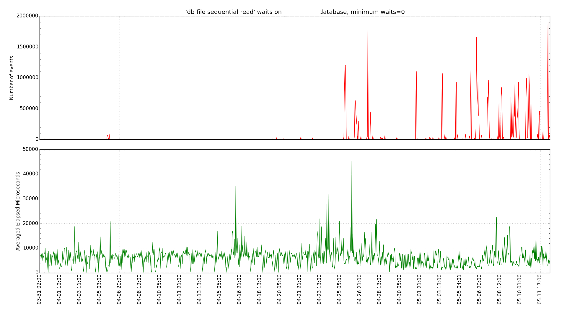
We did notice a high I/O time on the Linux executions. Running AWR reports showed about a 5 millisecond single block read time on Linux and about 1 millisecond on HP. I also graphed this over time using my Python scripts:

Linux db file sequential read (single block read) graph:

Linux

HP-UX db file sequential read graph:

HP

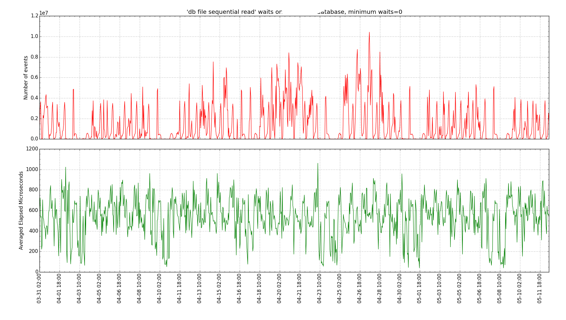
So, in general our source HP system was seeing sub millisecond single block reads but our new Linux system was seeing multiple millisecond reads. So, this lead us to look at differences in the storage system. It seems that the original system was on flash or solid state disk and the new one was not. So, we are going to move the new system to SSD and see how that affects the query performance.

Even though this led to a possible hardware issue I thought it was worth sharing the process I took to get there including eliminating differences in the query plan by matching the plan on the original platform.

Bobby

Postscript:

Our Linux and storage teams moved the new Linux VM to solid state disk and resolved these issues. The query ran about 10 times faster than it did on the original system after moving Linux to SSD.

HP Version:

END_INTERVAL_TIME         EXECUTIONS_DELTA Elapsed Average ms
------------------------- ---------------- ------------------
02.00.03.099 PM                        245         5341.99923 
03.00.15.282 PM                        250         1280.99632 
04.00.27.536 PM                        341         3976.65855 
05.00.39.887 PM                        125         2619.58894

Linux:

END_INTERVAL_TIME         EXECUTIONS_DELTA Elapsed Average ms
------------------------- ---------------- ------------------
16-MAY-16 09.00.35.436 AM              162         191.314809
16-MAY-16 10.00.38.835 AM              342         746.313994
16-MAY-16 11.00.42.366 AM              258         461.641705
16-MAY-16 12.00.46.043 PM              280         478.601618

The single block read time is well under 1 millisecond now that 
the Linux database is on SSD.

END_INTERVAL_TIME          number of waits ave microseconds 
-------------------------- --------------- ---------------- 
15-MAY-16 11.00.54.676 PM           544681       515.978687
16-MAY-16 12.00.01.873 AM           828539       502.911935
16-MAY-16 01.00.06.780 AM           518322       1356.92377
16-MAY-16 02.00.10.272 AM            10698       637.953543
16-MAY-16 03.00.13.672 AM              193       628.170984
16-MAY-16 04.00.17.301 AM              112        1799.3125
16-MAY-16 05.00.20.927 AM             1680       318.792262
16-MAY-16 06.00.24.893 AM              140       688.914286
16-MAY-16 07.00.28.693 AM             4837       529.759768
16-MAY-16 08.00.32.242 AM            16082       591.632508
16-MAY-16 09.00.35.436 AM           280927       387.293204
16-MAY-16 10.00.38.835 AM           737846        519.94157
16-MAY-16 11.00.42.366 AM          1113762       428.772997
16-MAY-16 12.00.46.043 PM           562258       510.357372

Sweet!

Posted in Uncategorized | Leave a comment

Comparing Common Queries Between Test and Production

The developers complained that their test database was so much slower than production that they could not use it to really test whether their batch processes would run fast enough when migrated to production. They did not give me any particular queries to check. Instead they said that the system was generally too slow. So, I went through a process to find SQL statements that they had run in test and that normally run in production and compare their run times. I thought that I would document the process that I went through here.

First I found the top 100 queries by elapsed time on both the test and production databases using this query:

column FORCE_MATCHING_SIGNATURE format 99999999999999999999

select FORCE_MATCHING_SIGNATURE from
(select
FORCE_MATCHING_SIGNATURE,
sum(ELAPSED_TIME_DELTA) total_elapsed
from DBA_HIST_SQLSTAT
where 
FORCE_MATCHING_SIGNATURE is not null and
FORCE_MATCHING_SIGNATURE <>0
group by FORCE_MATCHING_SIGNATURE
order by total_elapsed desc)
where rownum < 101;

The output looked like this:

FORCE_MATCHING_SIGNATURE
------------------------
      944718698451269965
     4634961225655610267
    15939251529124125793
    15437049687902878835
     2879196232471320459
    12776764566159396624
    14067042856362022182
...

Then I found the signatures that were in common between the two lists.

insert into test_sigs values (944718698451269965);
insert into test_sigs values (4634961225655610267);
insert into test_sigs values (15939251529124125793);
...
insert into prod_sigs values (3898230136794347827);
insert into prod_sigs values (944718698451269965);
insert into prod_sigs values (11160330134321800286);
...
select * from test_sigs
intersect
select * from prod_sigs;

This led to 32 values of FORCE_MATCHING_SIGNATURE which represented queries that ran on both test and production, except for the possible difference in constants.

Next I looked at the overall performance of these 32 queries in test and production using this query:

create table common_sigs
(FORCE_MATCHING_SIGNATURE number);

insert into common_sigs values (575231776450247964);
insert into common_sigs values (944718698451269965);
insert into common_sigs values (1037345866341698119);
...

select 
sum(executions_delta) total_executions,
sum(ELAPSED_TIME_DELTA)/(sum(executions_delta)*1000),
sum(CPU_TIME_DELTA)/(sum(executions_delta)*1000),
sum(IOWAIT_DELTA)/(sum(executions_delta)*1000),
sum(CLWAIT_DELTA)/(sum(executions_delta)*1000),
sum(APWAIT_DELTA)/(sum(executions_delta)*1000),
sum(CCWAIT_DELTA)/(sum(executions_delta)*1000),
sum(BUFFER_GETS_DELTA)/sum(executions_delta),
sum(DISK_READS_DELTA)/sum(executions_delta),
sum(ROWS_PROCESSED_DELTA)/sum(executions_delta)
from DBA_HIST_SQLSTAT ss,common_sigs cs
where 
ss.FORCE_MATCHING_SIGNATURE = cs.FORCE_MATCHING_SIGNATURE;

Here is part of the output:

TOTAL_EXECUTIONS Elapsed Average ms CPU Average ms IO Average ms
---------------- ------------------ -------------- -------------
         5595295         366.185529      241.92785    59.8682797
          430763         1273.75822     364.258421    1479.83294

The top line is production and the bottom is test.

This result supported the development team’s assertion that test was slower than production. The 32 queries averaged about 3.5 times longer run times in test than in production. Also, the time spent on I/O was about 25 times worse. I am not sure why the I/O time exceeded the elapsed time on test. I guess it has something to do with how Oracle measures I/O time. But clearly on average these 32 queries are much slower on test and I/O time probably caused most of the run time difference.

After noticing this big difference between test and production I decided to get these same sorts of performance metrics for each signature to see if certain ones were worse than others. The query looked like this:

select 
ss.FORCE_MATCHING_SIGNATURE,
sum(executions_delta) total_executions,
sum(ELAPSED_TIME_DELTA)/(sum(executions_delta)*1000),
sum(CPU_TIME_DELTA)/(sum(executions_delta)*1000),
sum(IOWAIT_DELTA)/(sum(executions_delta)*1000),
sum(CLWAIT_DELTA)/(sum(executions_delta)*1000),
sum(APWAIT_DELTA)/(sum(executions_delta)*1000),
sum(CCWAIT_DELTA)/(sum(executions_delta)*1000),
sum(BUFFER_GETS_DELTA)/sum(executions_delta),
sum(DISK_READS_DELTA)/sum(executions_delta),
sum(ROWS_PROCESSED_DELTA)/sum(executions_delta)
from DBA_HIST_SQLSTAT ss,common_sigs cs
where ss.FORCE_MATCHING_SIGNATURE = cs.FORCE_MATCHING_SIGNATURE
having 
sum(executions_delta) > 0
group by
ss.FORCE_MATCHING_SIGNATURE
order by
ss.FORCE_MATCHING_SIGNATURE;

I put together the outputs from running this query on test and production and lined the result up like this:

FORCE_MATCHING_SIGNATURE    PROD Average ms    TEST Average ms
------------------------ ------------------ ------------------
      575231776450247964         20268.6719         16659.4585
      944718698451269965         727534.558          3456111.6 *
     1037345866341698119         6640.87641         8859.53518
     1080231657361448615         3611.37698         4823.62857
     2879196232471320459         95723.5569         739287.601 *
     2895012443099075884         687272.949         724081.946
     3371400666194280661         1532797.66         761762.181
     4156520416999188213         109238.997         213658.722
     4634693999459450255          4923.8897         4720.16455
     5447362809447709021         2875.37308          2659.5754
     5698160695928381586         17139.6304         16559.1932
     6260911340920427003         290069.674         421058.874 *
     7412302135920006997         20039.0452         18951.6357
     7723300319489155163         18045.9756         19573.4784
     9153380962342466451         1661586.53         1530076.01
     9196714121881881832         5.48003488         5.13169472
     9347242065129163091         4360835.92         4581093.93
    11140980711532357629         3042320.88         5048356.99
    11160330134321800286         6868746.78         6160556.38
    12212345436143033196          5189.7972         5031.30811
    12776764566159396624         139150.231         614207.784  *
    12936428121692179551         3563.64537         3436.59365
    13637202277555795727          7360.0632         6410.02772
    14067042856362022182         859.732015         771.041714
    14256464986207527479         51.4042938         48.9237251
    14707568089762185958         627.586095          414.14762
    15001584593434987669         1287629.02         1122151.35
    15437049687902878835         96014.9782         996974.876  *
    16425440090840528197         48013.8912         50799.6184
    16778386062441486289         29459.0089         26845.8327
    17620933630628481201         51199.0511         111785.525  *
    18410003796880256802         581563.611         602866.609

I put an asterisk (*) beside the six queries that were much worse on test than production. I decided to focus on these six to get to the bottom of the reason between the difference. Note that many of the 32 queries ran about the same on test as prod so it really isn’t the case that everything was slow on test.

Now that I had identified the 6 queries I wanted to look at what they were spending their time on including both CPU and wait events. I used the following query to use ASH to get a profile of the time spent by these queries on both databases:

select 
case SESSION_STATE
when 'WAITING' then event
else SESSION_STATE
end TIME_CATEGORY,
(count(*)*10) seconds
from DBA_HIST_ACTIVE_SESS_HISTORY
where 
FORCE_MATCHING_SIGNATURE in
('944718698451269965',
'2879196232471320459',
'6260911340920427003',
'12776764566159396624',
'15437049687902878835',
'17620933630628481201')
group by SESSION_STATE,EVENT
order by seconds desc;

The profile looked like this in test:

TIME_CATEGORY            SECONDS
------------------------ -------
db file parallel read     207450
ON CPU                    141010
db file sequential read    62990
direct path read           36980
direct path read temp      29240
direct path write temp     23110

The profile looked like this in production:

TIME_CATEGORY            SECONDS
------------------------ -------
ON CPU                    433260
PX qref latch              64200
db file parallel read      35730
db file sequential read    14360
direct path read           12750
direct path write temp     12000

So, I/O waits dominate the time on test but not production. Since db file parallel read and db file sequential read were the top I/O waits for these 6 queries I used ash to see which of the 6 spent the most time on these waits.

db file parallel read:

select
  2  sql_id,
  3  (count(*)*10) seconds
  4  from DBA_HIST_ACTIVE_SESS_HISTORY
  5  where
  6  FORCE_MATCHING_SIGNATURE in
  7  ('944718698451269965',
  8  '2879196232471320459',
  9  '6260911340920427003',
 10  '12776764566159396624',
 11  '15437049687902878835',
 12  '17620933630628481201') and
 13  event='db file parallel read'
 14  group by sql_id
 15  order by seconds desc;

SQL_ID           SECONDS
------------- ----------
ak2wk2sjwnd34     159020
95b6t1sp7y40y      37030
brkfcwv1mqsas      11370
7rdc79drfp28a         30

db file sequential read:

select
  2  sql_id,
  3  (count(*)*10) seconds
  4  from DBA_HIST_ACTIVE_SESS_HISTORY
  5  where
  6  FORCE_MATCHING_SIGNATURE in
  7  ('944718698451269965',
  8  '2879196232471320459',
  9  '6260911340920427003',
 10  '12776764566159396624',
 11  '15437049687902878835',
 12  '17620933630628481201') and
 13  event='db file sequential read'
 14  group by sql_id
 15  order by seconds desc;

SQL_ID           SECONDS
------------- ----------
95b6t1sp7y40y      26840
ak2wk2sjwnd34      22550
6h0km9j5bp69t      13300
brkfcwv1mqsas        170
7rdc79drfp28a        130

Two queries stood out at the top waiters on these two events: 95b6t1sp7y40y and ak2wk2sjwnd34. Then I just ran my normal sqlstat query for both sql_ids for both test and production to find out when they last ran. Here is what the query looks like for ak2wk2sjwnd34:

select ss.sql_id,
ss.plan_hash_value,
sn.END_INTERVAL_TIME,
ss.executions_delta,
ELAPSED_TIME_DELTA/(executions_delta*1000) "Elapsed Average ms",
CPU_TIME_DELTA/(executions_delta*1000) "CPU Average ms",
IOWAIT_DELTA/(executions_delta*1000) "IO Average ms",
CLWAIT_DELTA/(executions_delta*1000) "Cluster Average ms",
APWAIT_DELTA/(executions_delta*1000) "Application Average ms",
CCWAIT_DELTA/(executions_delta*1000) "Concurrency Average ms",
BUFFER_GETS_DELTA/executions_delta "Average buffer gets",
DISK_READS_DELTA/executions_delta "Average disk reads",
ROWS_PROCESSED_DELTA/executions_delta "Average rows processed"
from DBA_HIST_SQLSTAT ss,DBA_HIST_SNAPSHOT sn
where ss.sql_id = 'ak2wk2sjwnd34'
and ss.snap_id=sn.snap_id
and executions_delta > 0
and ss.INSTANCE_NUMBER=sn.INSTANCE_NUMBER
order by ss.snap_id,ss.sql_id;

I found two time periods where both of these queries were recently run on both test and production and got an AWR report for each time period to compare them.

Here are a couple of pieces of the AWR report for the test database:

testtop5

testsqlelapsed

Here are similar pieces for the production database:

top5 foreground elapsed

What really stood out to me was that the wait events were so different. In production the db file parallel read waits averaged around 1 millisecond and the db file sequential reads averaged under 1 ms. On test they were 26 and 5 milliseconds, respectively. The elapsed times for sql_ids 95b6t1sp7y40y and ak2wk2sjwnd34 were considerably longer in test.

This is as far as my investigation went. I know that the slowdown is most pronounced on the two queries and I know that their I/O waits correspond to the two wait events. I am still trying to find a way to bring the I/O times down on our test database so that it more closely matches production. But at least I have a more narrow focus with the two top queries and the two wait events.

Bobby

Posted in Uncategorized | 8 Comments

Jonathan Lewis

I am finally getting around to finishing my four-part blog series on people who have had the most influence on my Oracle performance tuning work. The previous three people were Craig ShallahamerDon Burleson, and Cary Millsap. The last person is Jonathan Lewis. These four people, listed and blogged about in chronological order, had the most influence on my understanding of how to do Oracle database performance tuning. There are many other great people out there and I am sure that other DBAs would produce their own, different, list of people who influenced them. But this list reflects my journey through my Oracle database career and the issues that I ran into and the experiences that I had. I ran into Jonathan Lewis’ work only after years of struggling with query tuning and getting advice from others. I ran into his material right around the time that I was beginning to learn about how the Oracle optimizer worked and some of its limits. Jonathan was a critical next step in my understanding of how Oracle’s optimizer worked and why it sometimes failed to pick the most efficient way to run a query.

Jonathan has produced many helpful tuning resources including his blog, his participation in online forums, and his talks at user group conferences, but the first and most profound way he taught me about Oracle performance tuning was through his query tuning book Cost-Based Oracle Fundamentals. It’s $30 on Amazon and that is an incredibly small amount of money to pay compared to the value of the material inside the book. I had spent many hours over several years trying to understand why the Oracle optimizer some times choses the wrong way to run a query. In many cases the fast way to run something was clear to me and the optimizer’s choices left me stumped. The book helped me better understand how the Oracle optimizer chooses what it thinks is the best execution plan. Jonathan’s book describes the different parts of a plan – join types, access methods, etc. – and how the optimizer assigns a cost to the different pieces of a plan. The optimizer chooses the plan with the least cost, but if some mistake causes the optimizer to calculate an unrealistic cost then it might choose a poor plan. Understanding why the optimizer would choose a slow plan helped me understand how to resolve performance issues or prevent them from happening, a very valuable skill.

There is a lot more I could say about what I got from Jonathan Lewis’ book including just observing how he operated. Jonathan filled his book with examples which show concepts that he was teaching. I think that I have emulated the kind of building of test scripts that you see throughout his book and on his blog and community forums. I think I have emulated not only Jonathan’s approach but the approaches of all four of the people who I have spotlighted in this series. Each have provided me with profoundly helpful technical information that has helped me in my career. But they have also provided me with a pattern of what an Oracle performance tuning practitioner looks like. What kind of things do they do? To this point in my career I have found the Oracle performance tuning part of my job to be the most challenging and interesting and probably the most valuable to my employers. Jonathan Lewis and the three others in this four-part series have been instrumental in propelling me along this path and I am very appreciative.

Bobby

Posted in Uncategorized | 2 Comments

Log file parallel write wait graph

I got a chance to use my onewait Python based graph to help with a performance problem. I’m looking at slow write time from the log writer on Thursday mornings. Here is the graph with the database name erased:

log_file_parallel_write_waits

We are still trying to track down the source of the problem but there seems to be a backup on another system that runs at times that correspond to the spike in log file parallel write wait times. The nice thing about this graph is that it shows you activity on the top and average wait time on the bottom so you can see if the increased wait time corresponds to a spike in activity. In this case there does not seem to be any increase in activity on the problematic database.  But that makes sense if the real problem is contention by a backup on another system.

Anyway, my Python graphs are far from perfect but still helpful in this case.

Bobby

Posted in Uncategorized | Leave a comment

Python DBA Graphs Github Repository

I decided to get rid of the Github repository that I had experimented with and to create a new one. The old one had a dump of all my SQL scripts but without any documentation. But, I have updated my Python graphing scripts a bit at a time and have had some recent value from these scripts in my Oracle database tuning work. So, I created a Github repository called PythonDBAGraphs. I think it will be more valuable to have a repository that is more focused and is being actively updated and documented.

It is still very simple but I have gotten real value from the two graphs that are included.

Bobby

Posted in Uncategorized | Leave a comment

Another SQL Profile to the rescue!

We have had problems with set of databases over the past few weeks. Our team does not support these databases, but my director asked me to help. These are 11.2.0.1 Windows 64 bit Oracle databases running on Windows 2008. The incident reports said that the systems stop working and that the main symptom was that the oracle.exe process uses all the CPU. They were bouncing the database server when they saw this behavior and it took about 30 minutes after the bounce for the CPU to go back down to normal. A Windows server colleague told me that at some point in the past a new version of virus software had apparently caused high CPU from the oracle.exe process.

At first I looked for some known bugs related to high CPU and virus checkers without much success. Then I got the idea of just checking for query performance. After all, a poorly performing query can eat up a lot of CPU. These Windows boxes only have 2 cores so it would not take many concurrently running high CPU queries to max it out. So, I got an AWR report covering the last hour of a recent incident. This was the top SQL:

Top SQL

The top query, sql id 27d8x8p6139y6, stood out as very inefficient and all CPU. It seemed clear to me from this listing that the 2 core box had a heavy load and a lot of waiting for CPU queuing. %IO was zero but %CPU was only 31%. Most likely the rest was CPU queue time.

I also looked at my sqlstat report to see which plans 27d8x8p6139y6 had used over time.

PLAN_HASH_VALUE END_INTERVAL_TIME     EXECUTIONS Elapsed ms
--------------- --------------------- ---------- -----------
     3067874494 07-MAR-16 09.00.50 PM        287  948.102286
     3067874494 07-MAR-16 10.00.03 PM        292  1021.68191
     3067874494 07-MAR-16 11.00.18 PM        244  1214.96161
     3067874494 08-MAR-16 12.00.32 AM        276  1306.16222
     3067874494 08-MAR-16 01.00.45 AM        183  1491.31307
      467860697 08-MAR-16 01.00.45 AM        125      .31948
      467860697 08-MAR-16 02.00.59 AM        285  .234073684
      467860697 08-MAR-16 03.00.12 AM        279  .214354839
      467860697 08-MAR-16 04.00.25 AM        246   .17147561
      467860697 08-MAR-16 05.00.39 AM         18        .192
     2868766721 13-MAR-16 06.00.55 PM         89    159259.9
     3067874494 13-MAR-16 06.00.55 PM          8  854.384125
     2868766721 13-MAR-16 07.00.50 PM         70  1331837.56

Plan 2868766721 seemed terrible but plan 467860697 seemed great.

Our group doesn’t support these databases so I am not going to dig into how the application gathers statistics, what indexes it uses, or how the vendor designed the application. But, it seems possible that forcing the good plan with a SQL Profile could resolve this issue without having any access to the application or understanding of its design.

But, before plunging headlong into the use of a SQL Profile I looked at the plan and the SQL text.  I have edited these to hide any proprietary details:

SELECT T.*
    FROM TAB_MYTABLE1 T,
         TAB_MYTABLELNG A,
         TAB_MYTABLE1 PIR_T,
         TAB_MYTABLELNG PIR_A
   WHERE     A.MYTABLELNG_ID = T.MYTABLELNG_ID
         AND A.ASSIGNED_TO = :B1
         AND A.ACTIVE_FL = 1
         AND T.COMPLETE_FL = 0
         AND T.SHORTED_FL = 0
         AND PIR_T.MYTABLE1_ID = T.PIR_MYTABLE1_ID
         AND ((PIR_A.FLOATING_PIR_FL = 1 
               AND PIR_T.COMPLETE_FL = 1)
              OR PIR_T.QTY_PICKED IS NOT NULL)
         AND PIR_A.MYTABLELNG_ID = PIR_T.MYTABLELNG_ID
         AND PIR_A.ASSIGNED_TO IS NULL
ORDER BY T.MYTABLE1_ID

The key thing I noticed is that there was only one bind variable. The innermost part of the good plan uses an index on the column that the query equates with the bind variable. The rest of the plan is a nice nested loops plan with range and unique index scans. I see plans in this format in OLTP queries where you are looking up small numbers of rows using an index and join to related tables.

-----------------------------------------------------------------
Id | Operation                        | Name                     
-----------------------------------------------------------------
 0 | SELECT STATEMENT                 |                          
 1 |  SORT ORDER BY                   |                          
 2 |   NESTED LOOPS                   |                          
 3 |    NESTED LOOPS                  |                          
 4 |     NESTED LOOPS                 |                          
 5 |      NESTED LOOPS                |                          
 6 |       TABLE ACCESS BY INDEX ROWID| TAB_MYTABLELNG           
 7 |        INDEX RANGE SCAN          | AK_MYTABLELNG_BY_USER    
 8 |       TABLE ACCESS BY INDEX ROWID| TAB_MYTABLE1             
 9 |        INDEX RANGE SCAN          | AK_MYTABLE1_BY_MYTABLELNG
10 |      TABLE ACCESS BY INDEX ROWID | TAB_MYTABLE1             
11 |       INDEX UNIQUE SCAN          | PK_MYTABLE1              
12 |     INDEX UNIQUE SCAN            | PK_MYTABLELNG            
13 |    TABLE ACCESS BY INDEX ROWID   | TAB_MYTABLELNG           
-----------------------------------------------------------------

The bad plan had a gross Cartesian merge join:

Plan hash value: 2868766721

----------------------------------------------------------------
Id | Operation                       | Name                     
----------------------------------------------------------------
 0 | SELECT STATEMENT                |                          
 1 |  NESTED LOOPS                   |                          
 2 |   NESTED LOOPS                  |                          
 3 |    MERGE JOIN CARTESIAN         |                          
 4 |     TABLE ACCESS BY INDEX ROWID | TAB_MYTABLE1             
 5 |      INDEX FULL SCAN            | PK_MYTABLE1              
 6 |     BUFFER SORT                 |                          
 7 |      TABLE ACCESS BY INDEX ROWID| TAB_MYTABLELNG           
 8 |       INDEX RANGE SCAN          | AK_MYTABLELNG_BY_USER    
 9 |    TABLE ACCESS BY INDEX ROWID  | TAB_MYTABLE1             
10 |     INDEX RANGE SCAN            | AK_MYTABLE1_BY_MYTABLELNG
11 |   TABLE ACCESS BY INDEX ROWID   | TAB_MYTABLELNG           
12 |    INDEX RANGE SCAN             | AK_MYTABLELNG_BY_USER    
----------------------------------------------------------------

Reviewing the SQL made me believe that there was a good chance that a SQL Profile forcing the good plan would resolve the issue. Sure, there could be some weird combination of data and bind variable values that make the bad plan the better one. But, given that this was a simple transactional application it seems most likely that the straightforward nested loops with index on the only bind variable plan would be best.

We used the SQL Profile to force these plans on four servers and so far the SQL Profile has resolved the issues. I’m not saying that forcing a plan using a SQL Profile is the only or even best way to resolve query performance issues. But, this was a good example of where a SQL Profile makes sense. If modifying the application, statistics, parameters, and schema is not possible then a SQL Profile can come to your rescue in a heartbeat.

Bobby

Posted in Uncategorized | Leave a comment